Error Function and Effective Learning Rate
Step 6
This chapter explains simple neural networks and gradient computation. Although it’s somewhat beyond the main text, this is a good opportunity to summarize Chapter 7 of Bishop’s Deep Learning, so I’ll write about the differences in convergence behavior depending on the learning rate $\eta$.
Reference: Materials I created as a student (DL, Chapter 7)
Convergence of Error Functions
Local Quadratic Approximation Near the Minimum
Considering Taylor expansion near a point \(\mathbf{w}^*\) close to the minimum, we can approximate the error function using the Hessian matrix \(\mathbf{H}\):
\[E(\mathbf{w}) \approx E(\mathbf{w}^*) - \nabla E(\mathbf{w}^*)^{\mathrm T}(\mathbf{w}-\mathbf{w}^*) - \frac{1}{2}(\mathbf{w}-\mathbf{w}^*)^{\mathrm T}\mathbf{H}(\mathbf{w} - \mathbf{w}^*)\]Since the first derivative is 0 around the minimum,
\[E(\mathbf{w}) \approx E(\mathbf{w}^*) + \frac{1}{2}(\mathbf{w}-\mathbf{w}^*)^{\mathrm{T}}\mathbf{H}(\mathbf{w}-\mathbf{w}^*) \tag{1}\]Let’s see how the local shape (curvature) can be understood from this Hessian matrix.
Coordinate Transformation via Eigenvalues and Eigenvectors
Consider the eigenvalue problem of \(\mathbf{H}\):
\[\mathbf{H}\mathbf{u}_i = \lambda_i \mathbf{u}_i\]Expanding the deviation from the minimum in the eigenvector basis and defining \(\alpha_i\) as the quantity representing how far \(\mathbf{w}\) is from the minimum in the \(\mathbf{u}_i\) direction:
\[\mathbf{w}-\mathbf{w}^* = \sum_i \alpha_i \mathbf{u}_i \tag{2}\]Differentiating equation (1) with respect to \(\mathbf{w}\), the gradient under the quadratic approximation is expressed as:
\[\nabla E(\mathbf{w}) = \mathbf{H}(\mathbf{w}-\mathbf{w}^*) = \sum_i \lambda_i \alpha_i \mathbf{u}_i \tag{3}\]This shows that the gradient component in direction \(\mathbf{u}_i\) is \(\lambda_i \alpha_i\), meaning that directions with larger curvature \(\lambda_i\) have larger gradients for the same distance \(\alpha_i\).
From equation (2), the weight update equation can be written in the same basis as follows, showing that vector updates can be decomposed along each eigenvector axis:
\[\Delta\mathbf{w}=\sum_i \Delta\alpha_i \mathbf{u}_i \tag{4}\]From the above, since \(\alpha_i\) is a scalar in the direction of eigenvector \(\mathbf{u}_i\), by computing the projection of \((\mathbf{w}-\mathbf{w}^*)\) onto the eigenvector direction, we can write:
\[\mathbf{u}_i^{\mathrm{T}}(\mathbf{w}-\mathbf{w}^*)=\alpha_i\]Gradient Descent
Simple gradient descent can be written as:
\[\mathbf{w}^{(\tau)}=\mathbf{w}^{(\tau-1)}-\eta \nabla E(\mathbf{w}^{(\tau-1)})\]Combining this with the decomposition equations in the eigenvector directions computed in equations (3) and (4), we obtain for each direction:
\[\Delta\alpha_i = -\eta \lambda_i \alpha_i\]Therefore, the update equation for the deviation from the minimum \(\alpha\) is: \(\alpha_i^{\mathrm{new}}=\alpha_i^{\mathrm{old}}+\Delta\alpha_i = (1-\eta\lambda_i)\alpha_i^{\mathrm{old}} \tag{5}\)
Convergence Condition
From the update equation (5), we can see that the convergence condition for \(\alpha_i\) (condition to avoid divergence) is:
\[|1-\eta\lambda_i|<1 \tag{6}\]After \(T\) steps:
\[\alpha_i(T) = (1-\eta\lambda_i)^T\alpha_i(0)\]So as \(T\to\infty\), \(\alpha_i = \mathbf{w} - \mathbf{w}^* \to 0\), meaning \(\mathbf{w}\to\mathbf{w}^*\).
From condition (6), we obtain the following inequality:
\[-1 < 1-\eta\lambda_i < 1 \Longleftrightarrow 0 < \eta\lambda_i < 2 \Longleftrightarrow \eta < \frac{2}{\lambda_i}\]Near the minimum (local minimum), usually \(\lambda_i>0\), so to satisfy this simultaneously in all directions, we use the maximum eigenvalue \(\lambda_{\max}\):
\[\eta < \frac{2}{\lambda_{\max}}\]This shows how to set the constraint.
Convergence Speed
When we set \(\eta\) as large as possible with \(\eta=\frac{2}{\lambda_{\max}}\), the decay rate for each direction becomes:
\[\alpha_i(T)=\Bigl(1-\frac{2\lambda_i}{\lambda_{\max}}\Bigr)^T\alpha_i(0)\]The smallest update (= slowest) for \(\alpha_i\) occurs in the direction where \(\lambda_i\) is smallest, i.e., \(\lambda_{\min}\):
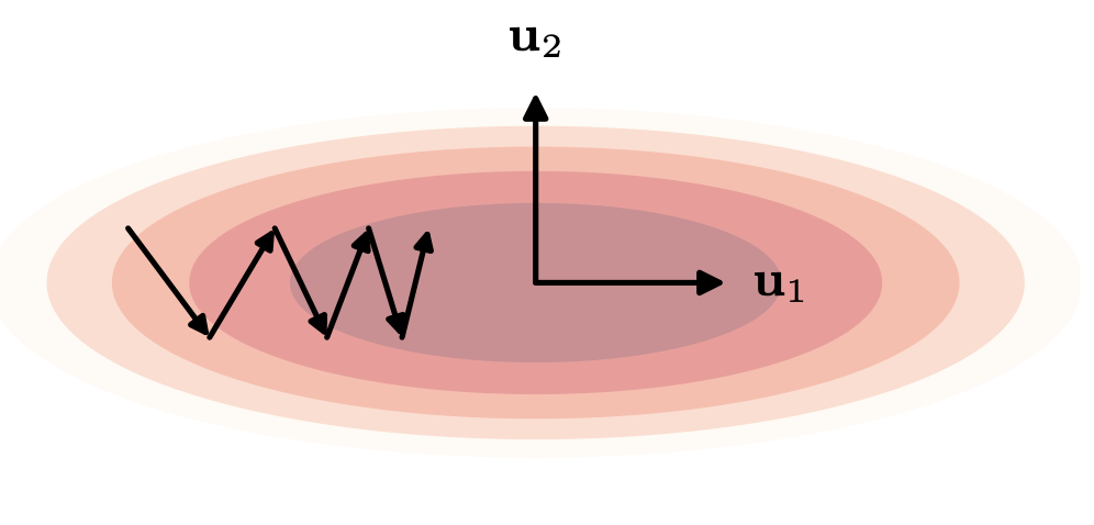
\[\alpha(T)=\Bigl(1-\frac{2\lambda_{\min}}{\lambda_{\max}}\Bigr)^T\alpha(0)\]This becomes the rate-limiting factor for convergence. The axis with small eigenvalues represents the direction where the deviation \(\mathbf{w} - \mathbf{w}^*\) in parameter space is hardest to update, corresponding to the long axis of the ellipse in parameter space (the flat direction with small gradient). From \(\frac{2\lambda_{\min}}{\lambda_{\max}}\), we can see that the larger the difference between the maximum and minimum eigenvalues, the slower the convergence.
[!Key point]
- See Deep Learning Figure 7.3
- \(\lambda_{\max}\) (steep gradient direction) determines the upper limit of \(\eta\)
- \(\lambda_{\min}\) (gentle gradient direction) determines the convergence speed
- The more elongated the valley (smaller \(\lambda_{\min}/\lambda_{\max}\)), the slower GD convergence becomes
Momentum
As discussed in the previous section, convergence becomes slow when \(\lambda_{\max}\) and \(\lambda_{\min}\) differ significantly. To address this, Momentum was proposed, which adds an inertia term to the movement in weight space to smooth out oscillations.
Update Equation
\[\Delta\mathbf{w}^{(\tau-1)} = -\eta\nabla E(\mathbf{w}^{(\tau-1)}) + \mu \Delta\mathbf{w}^{(\tau-2)} \tag{7}\]Here, \(\mu\) is the Momentum parameter (\(0\le \mu \le 1\)), which acts as inertia by mixing the previous update \(\Delta\mathbf{w}^{(\tau-2)}\) into the next update.
Effective Learning Rate
1. Smooth Slope
Consider a smooth slope where the curvature is small and the gradient remains constant. The situation where the gradient doesn’t change at any time step can be written as:
\[\nabla E(\mathbf{w}^{(\tau-1)})=\nabla E(\mathbf{w}^{(\tau-2)})=\cdots=\nabla E\]In this case, repeatedly substituting into the update equation (7):
\[\Delta\mathbf{w} = -\eta\nabla E,(1+\mu+\mu^2+\cdots)\]With \(\mid\mu\mid<1\) and the geometric series sum, the parameter update can be written as:
\[\Delta\mathbf{w} = -\frac{\eta}{1-\mu}\nabla E\]This means the effective learning rate increases from \(\eta \to \frac{\eta}{1-\mu}\). This shows that if the gradient direction remains the same, past updates accumulate in the same direction, accelerating the update speed.
2. Oscillating Region
On the other hand, in directions with large curvature like valley walls, GD tends to oscillate left and right. As an extreme example, consider the case where the gradient sign flips every step. In this case, the gradient at each time step becomes:
\[\nabla E(\mathbf{w}^{(\tau-1)})=-\nabla E(\mathbf{w}^{(\tau-2)})=\nabla E(\mathbf{w}^{(\tau-3)})=\cdots\]Applying the update equation (7) repeatedly as in the previous section and considering the geometric series with common ratio \(-\mu\):
\[\Delta\mathbf{w} = -\eta\nabla E,(1-\mu+\mu^2-\mu^3+\cdots) = -\frac{\eta}{1+\mu}\nabla E\]The effective learning rate becomes:
\[\frac{\eta}{1+\mu} < \eta\]This means that in directions where the gradient reverses (= oscillation directions), the inertia term cancels out the gradients, reducing the parameter update.
Summary
- Convergence condition: \(\mid1-\eta\lambda_i\mid<1\) must be satisfied in all directions, resulting in \(\eta < \frac{2}{\lambda_{\max}}\).
- Cause of slow convergence: Convergence speed is dominated by the slowest direction’s update \(\frac{\lambda_{\min}}{\lambda_{\max}}\).
- Momentum: Accelerates with effective learning rate \(\eta/(1-\mu)\) in consistent gradient directions, and decelerates with effective learning rate \(\eta/(1+\mu)\) in extreme oscillating directions.